Xarray's Rasterio Backend Tutorial

_toc.yml

@@ -86,6 +86,7 @@ parts:
         sections:
           - file: advanced/backends/1.Backend_without_Lazy_Loading.ipynb
           - file: advanced/backends/2.Backend_with_Lazy_Loading.ipynb
+          - file: advanced/backends/rasterio_backend.ipynb
       - file: advanced/accessors/accessors.md
         sections:
           - file: advanced/accessors/01_accessor_examples.ipynb

advanced/backends/rasterio_backend.ipynb

@@ -0,0 +1,289 @@
+{
+ "cells": [
+  {
+   "cell_type": "markdown",
+   "id": "0",
+   "metadata": {},
+   "source": [
+    "# Xarray's Rasterio backend\n",
+    "\n",
+    "In this lesson, we will learn how to use xarray's rasterio backend engine to open GeoTIFF rasters. By the end of the lesson, we will be able to:\n",
+    "\n",
+    ":::{admonition} Learning Goals\n",
+    "- Learn about the GeoTIFF format\n",
+    "- Lean about xarray's \"rasterio\" backend and the \"rioxarray\" accessor\n",
+    "- Learn how to read and plot GeoTIFF files with xarray\n",
+    "- Explore how to perform reprojection operations on rasters\n",
+    ":::\n",
+    "\n",
+    "## What are GeoTIFFs?\n",
+    "\n",
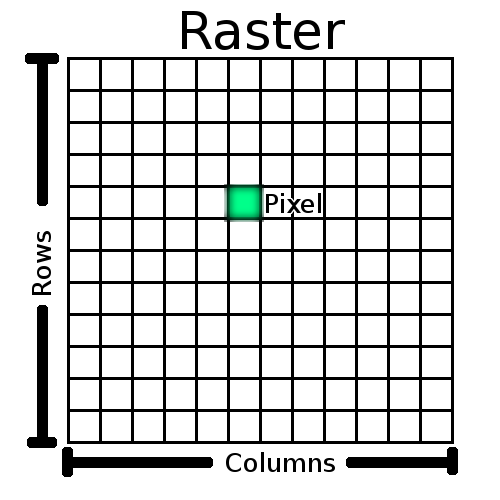
+    "The TIFF (Tagged Image File Format) format is a metadata rich image format for raster data. GeoTIFF (Geographic Tagged Image File Format) files are TIFF files that use georeferencing information (such as map projection and coordinate systems) as metadata. A GeoTIFF file with a single band contains 2D raster data for a single characteristic (i.e., variable) and maps to a geographic region. A GeoTIFF file can have multiple bands that all map to the same geographic region.\n",
+    "\n",
+    "![Raster_Image](https://docs.qgis.org/3.44/en/_images/raster_dataset.png)\n",
+    "\n",
+    "## Rasterio and Rioxarray Backends\n",
+    "\n",
+    "[Rasterio](https://rasterio.readthedocs.io/en/stable/intro.html) is a geospatial raster library that expresses GDAL ([Geospatial Data Abstraction Library](http://gdal.org)) data model with a Python API and CLI. [Rioxarray](https://corteva.github.io/rioxarray/stable/readme.html) is a wrapper around the rasterio library, that also extends the xarray api with the *rio* accessor. When you open a GeoTIFF file with the \"rasterio\" engine it returns the data as an xarray object with access to methods from the *rio* accessor.\n",
+    "\n"
+   ]
+  },
+  {
+   "cell_type": "markdown",
+   "id": "1",
+   "metadata": {},
+   "source": [
+    "## Reading a GeoTIFF\n",
+    "\n",
+    "Xarray's \"rasterio\" backend supports reading GeoTIFFs.\n",
+    "\n",
+    "Lets read a GeoTIFF file as an `xr.Dataset` by selecting `engine='rasterio'`"
+   ]
+  },
+  {
+   "cell_type": "code",
+   "execution_count": null,
+   "id": "2",
+   "metadata": {},
+   "outputs": [],
+   "source": [
+    "import xarray as xr"
+   ]
+  },
+  {
+   "cell_type": "code",
+   "execution_count": null,
+   "id": "3",
+   "metadata": {},
+   "outputs": [],
+   "source": [
+    "rds = xr.tutorial.open_dataset(\"RGB.byte.tif\", engine=\"rasterio\")"
+   ]
+  },
+  {
+   "cell_type": "markdown",
+   "id": "4",
+   "metadata": {},
+   "source": [
+    ":::{note} We can also read GeoTIFFs with `rioxarray.open_rasterio`.\n",
+    "\n",
+    "The following code snippet opens a GeoTIFF and returns a `DataArray` object\n",
+    "```python\n",
+    "import rioxarray\n",
+    "rioxarray.open_rasterio(\"RGB.byte.tif\")\n",
+    "```\n",
+    "\n",
+    ":::"
+   ]
+  },
+  {
+   "cell_type": "markdown",
+   "id": "5",
+   "metadata": {},
+   "source": [
+    "## Raster bands\n",
+    "\n",
+    "GeoTIFFS can have multiple bands each representing a range or band in the electromagnetic spectrum. Arrays stored within bands in xarray are data variables and `DataArray`'s objects in the the Xarray Data Model."
+   ]
+  },
+  {
+   "cell_type": "markdown",
+   "id": "6",
+   "metadata": {},
+   "source": [
+    "Lets get the `DataArray` object (or variable) from our dataset. The variable name is \"band_data\"."
+   ]
+  },
+  {
+   "cell_type": "code",
+   "execution_count": null,
+   "id": "7",
+   "metadata": {},
+   "outputs": [],
+   "source": [
+    "rda = rds[\"band_data\"]\n",
+    "rda"
+   ]
+  },
+  {
+   "cell_type": "markdown",
+   "id": "8",
+   "metadata": {},
+   "source": [
+    "Lets try getting the total number of bands for this GeoTIFF. Since `rioxarray` extends xarray with the *rio* accessor we can this accessor be able use many of the builtin `rasterio` methods."
+   ]
+  },
+  {
+   "cell_type": "code",
+   "execution_count": null,
+   "id": "9",
+   "metadata": {},
+   "outputs": [],
+   "source": [
+    "rda.rio.count"
+   ]
+  },
+  {
+   "cell_type": "markdown",
+   "id": "10",
+   "metadata": {},
+   "source": [
+    "### Selection by bands\n",
+    "We can also select by bands. Since there are 3 bands in this dataset we can return raster array for the first band of this `xr.DataArray` by with indexing\n",
+    "\n",
+    "Lets get the first band of this dataset and try plotting it"
+   ]
+  },
+  {
+   "cell_type": "code",
+   "execution_count": null,
+   "id": "11",
+   "metadata": {},
+   "outputs": [],
+   "source": [
+    "rda[0].plot(cmap=\"pink\")"
+   ]
+  },
+  {
+   "cell_type": "markdown",
+   "id": "12",
+   "metadata": {},
+   "source": [
+    "## Bounds\n",
+    "With `.rio.bounds()` we can get the spatial bounding box of our `DataArray`"
+   ]
+  },
+  {
+   "cell_type": "code",
+   "execution_count": null,
+   "id": "13",
+   "metadata": {},
+   "outputs": [],
+   "source": [
+    "rda.rio.bounds()"
+   ]
+  },
+  {
+   "cell_type": "markdown",
+   "id": "14",
+   "metadata": {},
+   "source": [
+    "## Transformation\n",
+    "\n",
+    "With `.rio.transform()` we can get the affine transformation matrix that maps pixel locations in (col, row) coordinates to (x, y) spatial positions.\n"
+   ]
+  },
+  {
+   "cell_type": "code",
+   "execution_count": null,
+   "id": "15",
+   "metadata": {},
+   "outputs": [],
+   "source": [
+    "rda.rio.transform()"
+   ]
+  },
+  {
+   "cell_type": "markdown",
+   "id": "16",
+   "metadata": {},
+   "source": [
+    "### Coordinate Reference System (CRS)\n",
+    "We `rio.crs` we can get the CRS of our raster and reproject our raster."
+   ]
+  },
+  {
+   "cell_type": "code",
+   "execution_count": null,
+   "id": "17",
+   "metadata": {},
+   "outputs": [],
+   "source": [
+    "rda.rio.crs"
+   ]
+  },
+  {
+   "cell_type": "markdown",
+   "id": "18",
+   "metadata": {},
+   "source": [
+    "### Reprojection\n",
+    "We can also reproject our raster from one CRS to another.\n",
+    "\n",
+    "Lets reproject our raster from \"EPSG:6326\" to \"EPSG:32612\""
+   ]
+  },
+  {
+   "cell_type": "code",
+   "execution_count": null,
+   "id": "19",
+   "metadata": {},
+   "outputs": [],
+   "source": [
+    "rda_reproj = rda.rio.reproject(\"EPSG:32612\")"
+   ]
+  },
+  {
+   "cell_type": "markdown",
+   "id": "20",
+   "metadata": {},
+   "source": [
+    ":::{note}\n",
+    "We have to update our CRS system to the new projection with `rio.write_crs`. We set `inplace=True` to write the CRS to the existing dataset."
+   ]
+  },
+  {
+   "cell_type": "code",
+   "execution_count": null,
+   "id": "21",
+   "metadata": {},
+   "outputs": [],
+   "source": [
+    "rda_reproj.rio.write_crs(\"EPSG:32612\", inplace=True)"
+   ]
+  },
+  {
+   "cell_type": "markdown",
+   "id": "22",
+   "metadata": {},
+   "source": [
+    "## Exercise"
+   ]
+  },
+  {
+   "cell_type": "markdown",
+   "id": "23",
+   "metadata": {},
+   "source": [
+    "::::{admonition} Exercise\n",
+    ":class: tip\n",
+    "\n",
+    "Can you reproject and update the CRS of second band of data to 'ESPG:3857' and plot your results?\n",
+    "\n",
+    ":::{admonition} Solution\n",
+    ":class: dropdown\n",
+    "\n",
+    "```python\n",
+    "rda[1].rio.reproject(\"EPSG:3857\").rio.write_crs(\"EPSG:3857\", inplace=True).plot()\n",
+    "```\n",
+    ":::\n",
+    "::::\n"
+   ]
+  }
+ ],
+ "metadata": {
+  "language_info": {
+   "codemirror_mode": {
+    "name": "ipython",
+    "version": 3
+   },
+   "file_extension": ".py",
+   "mimetype": "text/x-python",
+   "name": "python",
+   "nbconvert_exporter": "python",
+   "pygments_lexer": "ipython3"
+  }
+ },
+ "nbformat": 4,
+ "nbformat_minor": 5
+}